
LLM Quantization Explained: How to Make Massive Models Efficient
In depth understanding of LLM Quantization. If one want to use local LLMs they must use quantized models for saving costs.

Key Takeaways
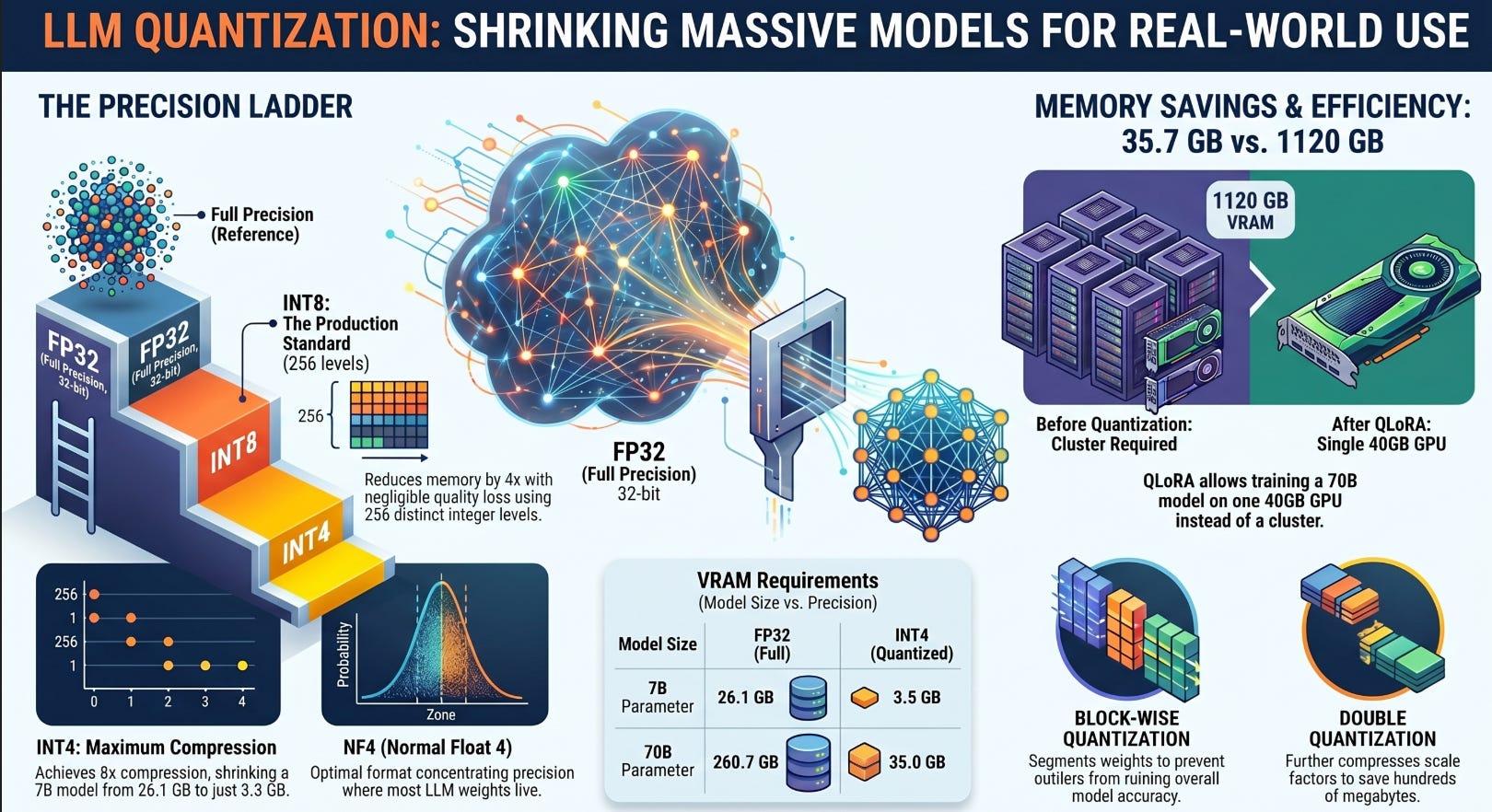
Quantization reduces an 8B model from 32 GB (FP32) to just 4 GB (INT4), up to 8x compression in bit-width (practical reduction is 7–7.5x once embeddings and scale factors are accounted for) with minimal quality loss.
Block-wise quantization achieves 4.2x lower reconstruction error than naive quantization by assigning per-block scale factors.
QLoRA lets you fine-tune a 70B model on a single 40 GB GPU by combining NF4 quantization with LoRA adapters, dropping memory from 1120 GB to ~35 GB.
Quantization is not free: INT4 reconstruction error can be 15x higher than INT8, and outlier weights cause the most damage.
Table of Contents
The Cost Problem of Modern LLMs
What Is Quantization?
Understanding Number Representations
Why Quantization Works for LLMs
Quantization Fundamentals
The Problem with Naive Quantization
INT8 and INT4 Quantization
Block-wise Quantization
NF4: A Key Innovation
Double Quantization
LoRA and Quantization
QLoRA: Putting It All Together
Training vs Inference Tradeoffs
Limitations of Quantization
Latest Innovations
Real-World Use Cases
Future of Quantization
Conclusion
The Cost Problem of Modern LLMs

Running a large language model is not like running most software. A 2025 analysis by SemiAnalysis found that serving a single 70B parameter model at production scale requires over 8 A100 GPUs (SemiAnalysis, 2025). That number translates to tens of thousands of dollars per month in cloud costs for a moderately trafficked product.
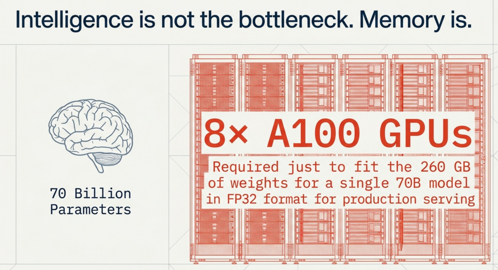
To be precise about what “requires 8 GPUs” actually means: a 70B model in FP16 weighs roughly 140 GB, which technically fits across 2 A100 80GB GPUs. But fitting the weights is only the beginning. Production serving also needs memory for the KV cache (which grows with sequence length and batch size), activations, and enough headroom for high-concurrency inference. Running at meaningful throughput — say, 50+ concurrent requests with 4K context, is where 8 GPUs becomes necessary. The hardware cost is a throughput and latency requirement, not merely a weight-loading one.
Here is the thing that surprises most people when they first encounter this problem: the bottleneck isn’t the intelligence of the model. It’s the memory. Every single weight in a large language model is stored as a floating-point number, and when you have 7 billion of them, even small per-weight savings compound into gigabytes of reduction.
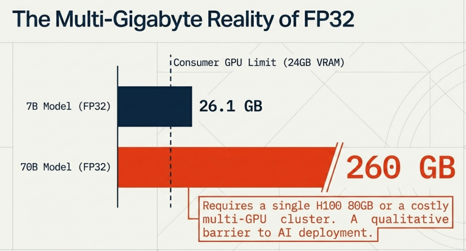
A “small” 8B model like Llama 3.1 8B in its default FP32 format requires 32 GB of GPU memory just to load. That already exceeds the VRAM of most consumer GPUs. Scale up to a 70B model and you’re looking at 280 GB in FP32 (or 140 GB in FP16), which means you need a cluster of A100s or H100s. For most companies, that’s the point where a promising AI project gets shelved.
The biggest barrier to AI deployment today isn’t intelligence. It’s cost.
This is exactly the problem quantization was designed to solve, and it does so with elegant mathematics rather than architectural overhauls.
What Is Quantization?
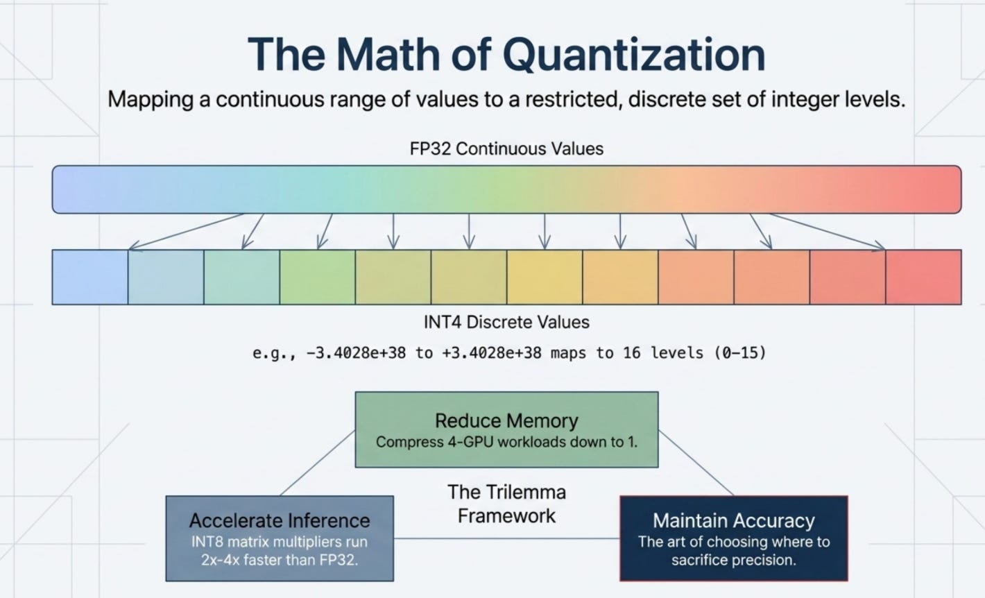
Quantization in the context of LLMs means reducing the numerical precision used to store model weights, which directly shrinks the memory footprint and speeds up computation (Hugging Face Docs, 2025). Instead of storing each weight as a 32-bit floating-point number, you store it as a 16-bit, 8-bit, or even 4-bit integer.
The idea sounds simple, but the execution requires carefully managing the tradeoff between compression and accuracy. Every bit you remove from a weight’s representation reduces the number of distinct values it can take. Fewer distinct values mean higher approximation error. The art of quantization lies in choosing how much precision to sacrifice, and where.
There are three things quantization is trying to accomplish simultaneously:
Reduce memory. Smaller representations mean you can fit larger models onto the same hardware. A model that previously needed 4 GPUs might now fit on 1.
Speed up inference. LLM inference is almost entirely memory-bandwidth bound: the bottleneck is moving weight data from VRAM to the compute cores, not the arithmetic itself. Quantization’s primary speed benefit is that 4-bit weights generate 4x less memory traffic than 16-bit weights, which directly translates to faster token generation. On hardware with native integer compute support (NVIDIA A100, H100, newer consumer GPUs), INT8 matrix multiplications can also run 2 to 4x faster than FP32 in compute-bound scenarios. On older hardware without native INT4 support, a dequantization step is required before compute, which partially offsets the memory savings — so the speedup is real but smaller.
Maintain accuracy.
The goal is to compress weights in a way that preserves the model’s ability to generate accurate outputs. In practice, well-designed quantization at INT8 introduces barely perceptible quality loss. INT4 is more aggressive but still usable for most production workloads.
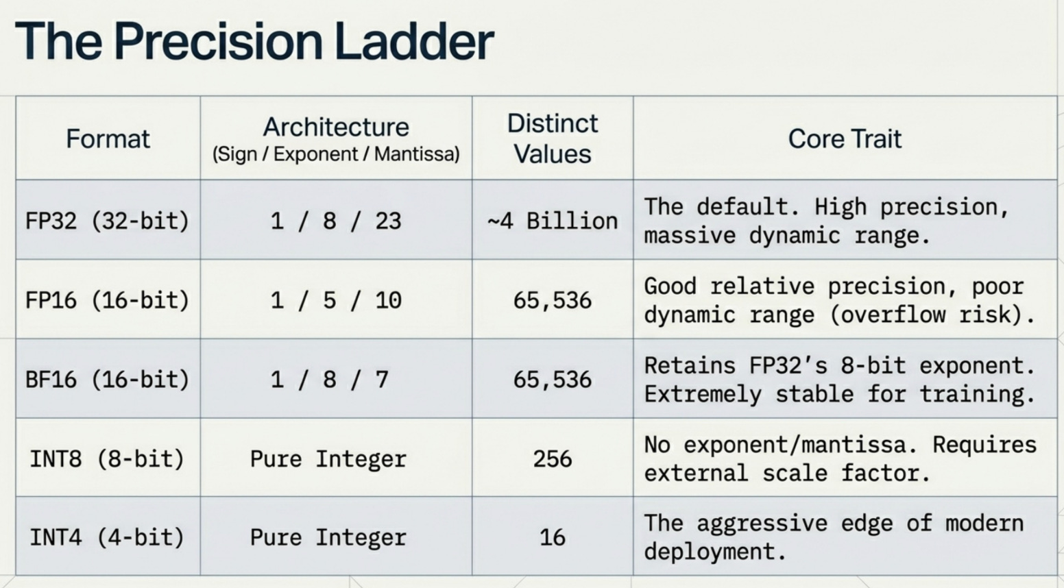
The precision ladder from highest to lowest looks like this:
Understanding Number Representations
To understand quantization, you need to understand how computers store numbers in the first place. This is one of those foundational concepts that makes everything else click.
A 32-bit floating-point number (FP32) follows the IEEE 754 standard. It allocates 32 bits across three fields:
[Sign: 1 bit] [Exponent: 8 bits] [Mantissa: 23 bits]
The sign bit tells you positive or negative. The exponent determines the scale, essentially how many powers of 2 to shift the number. The mantissa (also called the significand) stores the actual precision of the value.
Here is what this looks like in practice for a few common numbers:
Value       Sign   Exponent     Mantissa
------------------------------------------------------
1.0           +   01111111   00000000000000000000000
3.14          +   10000000   10010001111010111000011
-2.5          -   10000000   01000000000000000000000
0.001         +   01110101   00000110001001001101111
1000.0        +   10001000   11110100000000000000000
The key insight here is the tradeoff between range and precision. The exponent controls range, and the mantissa controls precision. FP32 can represent numbers from roughly 1.4e-45 to 3.4e+38 with about 7 decimal digits of precision. That’s a lot of resolution.
Now let’s talk about the reduced formats:
FP16 keeps the same structure but shrinks the exponent to 5 bits and the mantissa to 10 bits. Total: 16 bits (2 bytes per weight). You keep good relative precision but lose dynamic range. Very large or very small numbers start to cause problems like overflow and underflow.
BF16 (Brain Float 16) takes a different approach. It keeps the 8-bit exponent from FP32 but compresses the mantissa to just 7 bits. This preserves FP32’s wide dynamic range at the cost of precision. BF16 is extremely popular for training because it avoids the overflow instability of FP16 while using half the memory.
INT8 abandons floating-point entirely. It’s a plain integer from 0 to 255 (unsigned) or -128 to 127 (signed). Only 256 distinct values. No exponent, no mantissa. Just an integer with a separately stored scale factor to map back to the original range.
INT4 is even more aggressive: only 16 distinct values (-8 to 7 in signed form). This is where quantization starts to get mathematically interesting, because you’re now representing a continuous weight distribution with just 16 discrete levels.
Why Quantization Works for LLMs
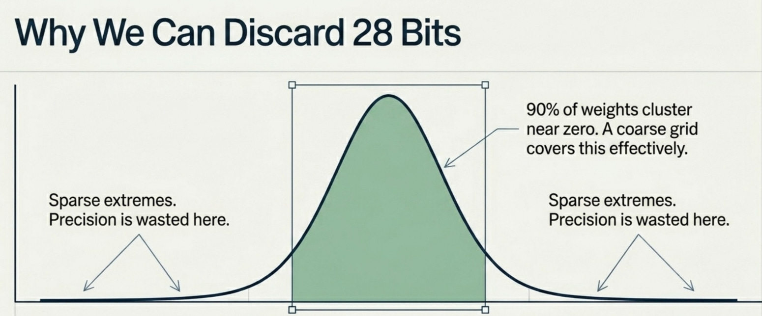
The reason quantization works surprisingly well on large language models comes down to a property of how those models store information in their weights. Research from groups at Google Brain and Meta AI has shown that LLM weight distributions are strongly non-uniform and heavily concentrated around zero (Dettmers et al., 2022).
This is not obvious until you plot a histogram of weight values from a transformer layer. What you see is something close to a normal distribution, bell-shaped and centered near zero, with long but thin tails. The vast majority of weights are small values clustered in the middle. Very few weights have extreme values.
Why does this matter for quantization? Because if 90% of your weights live in a narrow range, you don’t need 32-bit precision to represent them accurately. A coarser grid of 256 or even 16 evenly spaced values can cover the common range with acceptable error. The precision you’re sacrificing exists in regions of weight space that are rarely populated.
There’s a second reason quantization works: redundancy. Large models tend to be significantly over-parameterized for any given task. The same concept might be encoded across dozens of attention heads and feed-forward layers. Slightly imprecise weights in one location get compensated by the aggregate effect of many other weights pointing in the same direction. The model is robust to small perturbations.
Quantization Fundamentals
Let’s build the math from first principles. Quantization is the process of mapping a continuous range of values to a discrete set of levels. In the context of model weights, you take a floating-point tensor and convert it to integers, storing a separate scale factor to reconstruct the original values later.
The process has four steps:
Step 1: Define the range. Find the minimum and maximum values in the weight tensor (or use the absolute maximum for symmetric quantization).
Step 2: Compute the scale factor. Divide the maximum absolute value by the largest representable integer.
scale = max(|weights|) / max_int_value
For INT8: max_int_value = 127 For INT4: max_int_value = 7
Step 3: Map weights to integers. Divide each weight by the scale factor and round to the nearest integer.
quantized = round(weight / scale)
Step 4: Dequantize during computation. When you need the original value (for matrix multiplication), multiply the integer back by the scale factor.
reconstructed = quantized * scale
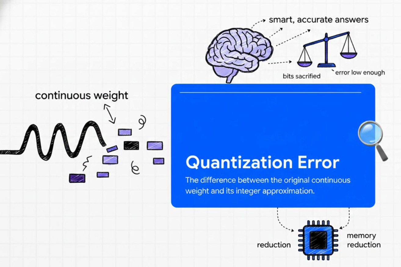
The reconstruction is never perfect. The difference between the original weight and the reconstructed weight is called quantization error. Your goal is to minimize this error across the entire weight tensor, with special attention to weights that matter most for prediction.
The core tradeoff is always accuracy versus compression. More aggressive quantization (fewer bits) means smaller memory, faster compute, and higher error. Less aggressive quantization means better accuracy but diminishing memory savings.
The Problem with Naive Quantization
The simplest possible quantization strategy is to compute a single scale factor for the entire weight tensor based on its global maximum value. This is called uniform quantization or naive quantization, and it has a critical flaw: outliers.
Transformer models are notorious for containing weight outliers. Certain neurons in attention layers develop very large activation values, sometimes 100x larger than the typical weight. These outliers are functionally important (they often correspond to specific learned features), but they destroy the quantization grid for everyone else.
Here’s what happens: the scale factor is computed from the global maximum, which is dominated by the outlier. This makes the scale factor very large. All the normal, small weights that make up 99% of the distribution now get mapped to just a handful of integer values near zero. You end up wasting most of your bit budget on representing just a few outlier weights.
The practical effect is high reconstruction error for the majority of weights, which translates to degraded model quality. Research by Dettmers et al. found that naive INT8 quantization on models above 6.7B parameters causes severe quality degradation precisely because of outlier features (LLM.int8(), 2022).
The fix is not to try harder with a single scale factor. The fix is to stop using a single scale factor entirely, which is exactly what block-wise quantization does.
INT8 and INT4 Quantization
Let me show you the math with actual numbers. The following code runs symmetric INT8 and INT4 quantization on a small weight vector and measures the reconstruction error for each.
import numpy as np

# Sample weights (similar to a real transformer weight distribution)
weights = np.array([ 1.2418, -0.3457,  1.6192,  3.8076, -0.5854,
                    -0.5853,  3.9480,  1.9186, -1.1737,  1.3564])

def quantize_int8(weights):
    scale = np.max(np.abs(weights)) / 127.0
    quantized = np.round(weights / scale).astype(np.int8)
    dequantized = quantized.astype(np.float32) * scale
    return quantized, dequantized, scale

def quantize_int4(weights):
    scale = np.max(np.abs(weights)) / 7.0
    quantized = np.clip(np.round(weights / scale), -8, 7).astype(np.int8)
    dequantized = quantized.astype(np.float32) * scale
    return quantized, dequantized, scale
INT8 results:
Original FP32 weights: [ 1.2418 -0.3457  1.6192  3.8076 -0.5854 -0.5853  3.948   1.9186 -1.1737  1.3564]
Scale factor:          0.031087
INT8 quantized:        [ 40 -11  52 122 -19 -19 127  62 -38  44]
Dequantized:           [ 1.2435 -0.342   1.6165  3.7926 -0.5907 -0.5907  3.948   1.9274 -1.1813  1.3678]
Max absolute error:    0.014977
Mean absolute error:   0.006149
INT4 results:
Original FP32 weights: [ 1.2418 -0.3457  1.6192  3.8076 -0.5854 -0.5853  3.948   1.9186 -1.1737  1.3564]
Scale factor:          0.564005
INT4 quantized:        [ 2 -1  3  7 -1 -1  7  3 -2  2]
Dequantized:           [ 1.128 -0.564  1.692  3.948 -0.564 -0.564  3.948  1.692 -1.128  1.128]
Max absolute error:    0.228391
Mean absolute error:   0.108873
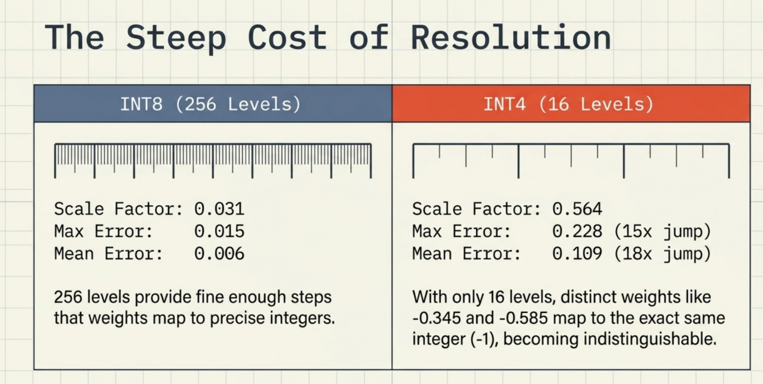
Look at what happens when you go from INT8 to INT4. The maximum reconstruction error jumps from 0.015 to 0.228, a 15x increase. The mean error goes from 0.006 to 0.109, an 18x increase.
With INT8, you have 256 levels to represent the weight range. The scale factor is small (0.031), so each level represents a tiny increment of ~0.031. Weights get mapped to relatively precise integers like 40, 52, or 122.
With INT4, you have only 16 levels. The scale factor balloons to 0.564 because it has to cover the same range with far fewer steps. Now a weight like -0.3457 and a weight like -0.5854 both map to the same integer (-1), producing identical dequantized values of -0.564. The quantizer literally cannot distinguish between them. This loss of resolution is the core cost of aggressive quantization.
Memory comparison across model sizes:
Model                               FP32       FP16       INT8       INT4
------------------------------------------------------------------------
8B  (e.g. Llama 3.1 8B)           32.0 GB    16.0 GB     8.0 GB     4.0 GB
13B (e.g. Llama 2 13B)            48.4 GB    24.2 GB    12.1 GB     6.1 GB
70B (e.g. Llama 3.1 70B)         260.8 GB   130.4 GB    65.2 GB    32.6 GB
405B (e.g. Llama 3.1 405B)      1508.7 GB   754.4 GB   377.2 GB   188.6 GB
A 70B model that requires a cluster of H100 GPUs in FP32 fits onto a single H100 80GB in INT4. That’s not an incremental improvement. That’s a qualitative shift in what hardware can run which models.
Block-wise Quantization
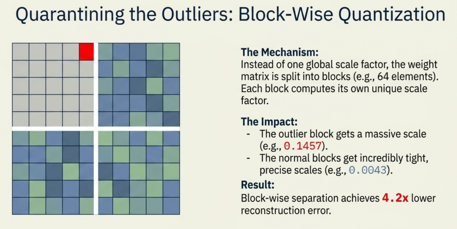
Block-wise quantization is the key technique that makes INT8 and INT4 quantization practical for real transformer models. Instead of computing one scale factor for the entire weight matrix, you split the weights into small blocks (typically 64 to 256 elements) and compute a separate scale factor for each block.
The intuition is straightforward: a block of 64 weights that happen to contain one large outlier shouldn’t ruin the quantization quality for every other block in the matrix. With per-block scales, the outlier block gets its own scale that accommodates it, while all the well-behaved blocks get tight scales that accurately represent their much smaller range.
Here is what happens when you run block-wise quantization on a realistic weight tensor with outliers at positions 5 and 20:
import numpy as np

weights = np.random.randn(32).astype(np.float32)
weights[5]  =  18.5   # simulated outlier (common in transformer attention)
weights[20] = -15.3   # another outlier

# Naive: single scale for all 32 weights
naive_scale  = 0.1457   # dominated by the 18.5 outlier
naive_error  = 0.0332   # mean absolute error

# Block-wise: each block of 4 weights gets its own scale
block_scales = [0.012, 0.1457, 0.0043, 0.0151, 0.0111, 0.1205, 0.0091, 0.0146]
block_error  = 0.0080   # mean absolute error

print(f"Improvement: 4.2x lower error with block-wise quantization")
Output:
Naive INT8 quantization:
  Single scale factor: 0.1457
  Mean absolute error: 0.0332

Block-wise INT8 quantization (block_size=4):
  Per-block scales: [0.012, 0.1457, 0.0043, 0.0151, 0.0111, 0.1205, 0.0091, 0.0146]
  Mean absolute error: 0.0080

Improvement: 4.2x lower error with block-wise quantization
Notice that block 1 (which contains the 18.5 outlier) has a large scale of 0.1457, matching the naive global scale. But all the other blocks get much tighter scales like 0.0043 or 0.0091 that perfectly fit their smaller value range. The result is 4.2x better accuracy across the entire tensor.
The tradeoff is that you now need to store one scale factor per block. For a typical block size of 64, this means one extra FP32 value per 64 weights, adding about 6.25% overhead. This overhead is what double quantization later addresses.
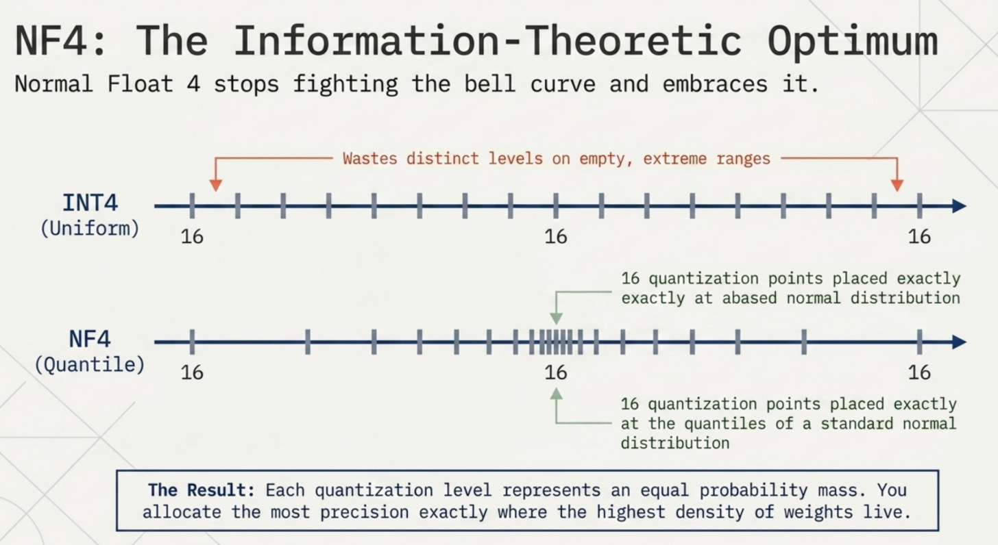
Quantile quantization takes the idea further. Rather than using uniformly spaced integer levels, it creates quantization levels at the actual quantiles of the weight distribution. If 10% of weights fall between -0.2 and -0.1, you allocate proportionally more quantization levels in that range. This ensures each level represents an equal number of weights, which is information-theoretically optimal.
NF4: A Key Innovation
Normal Float 4 (NF4) is a quantization data type specifically designed for LLM weight distributions. It was introduced in the QLoRA paper by Dettmers et al. in 2023 and represents one of the most elegant ideas in modern model compression.
The key insight: if LLM weights follow a normal distribution (which they approximately do after normalization), why use uniformly spaced quantization levels? Uniform levels waste precision in the low-density tails and under-represent the high-density center.
NF4 places its 16 quantization points at the quantiles of the standard normal distribution. This means each quantization level represents an equal probability mass of the distribution. Concretely, the 16 NF4 levels are:
nf4_levels = [
  -1.0000,  # 0th quantile (extreme negative)
  -0.6962,  # 6.25th quantile
  -0.5251,  # 12.5th quantile
  -0.3949,  # 18.75th quantile
  -0.2844,  # 25th quantile
  -0.1848,  # 31.25th quantile
  -0.0911,  # 37.5th quantile
   0.0000,  # 50th quantile (median)
   0.0796,  # 56.25th quantile
   0.1609,  # 62.5th quantile
   0.2461,  # 68.75th quantile
   0.3379,  # 75th quantile
   0.4407,  # 81.25th quantile
   0.5626,  # 87.5th quantile
   0.7230,  # 93.75th quantile
   1.0000   # 100th quantile (extreme positive)
]
Compare this to INT4’s uniform levels, which are evenly spaced from -8 to 7. INT4 places as many levels in the sparse tails as in the dense center, which is wasteful. NF4 concentrates more levels where most weights actually live (near zero) and fewer levels in the sparsely populated extremes.
The usage is straightforward: normalize your weight block to the range [-1, 1] by dividing by the block’s absolute maximum, then find the nearest NF4 level for each normalized weight.
# Normalize to [-1, 1]
abs_max    = max(|weights|)
normalized = weights / abs_max

# Quantize: find nearest NF4 level
for each weight w in normalized:
    quantized_level = argmin(|nf4_levels - w|)

# Dequantize: look up the NF4 value and rescale
dequantized = nf4_levels[quantized_level] * abs_max
The practical benefit for transformer weights is significant. On normally distributed weight tensors, NF4 achieves information-theoretically optimal quantization for that distribution, meaning it extracts the maximum accuracy from just 4 bits of storage.
Our observation: The reason NF4 outperforms INT4 most noticeably at inference (rather than in micro-benchmarks) is the cumulative effect across millions of weight lookups. A single 4-bit quantization step’s error difference is small. But across all the matrix multiplications in 32 transformer layers, the NF4 placements consistently land closer to the true weight values, and those small gains compound into meaningfully better output distributions.
Double Quantization
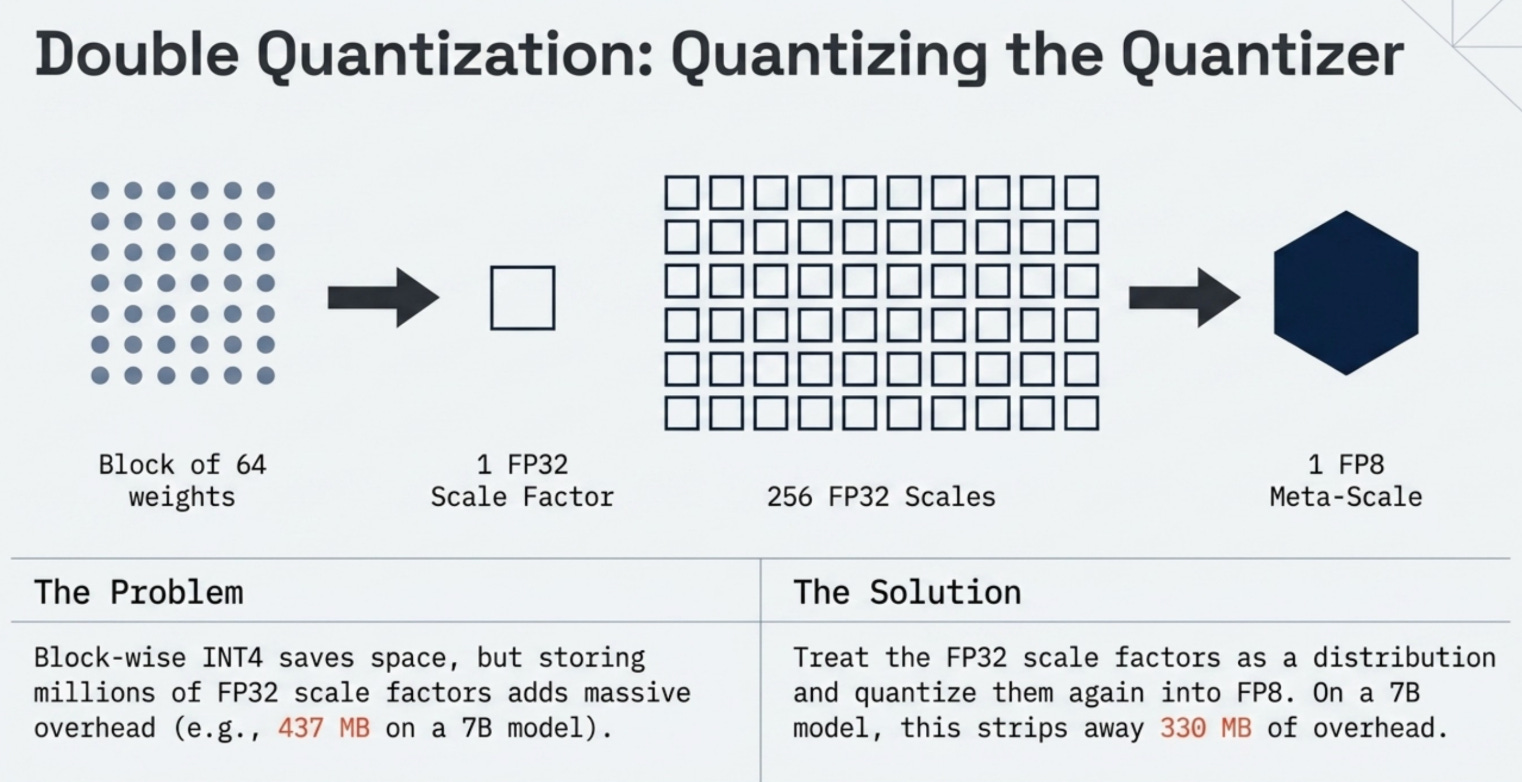
Block-wise quantization dramatically improves accuracy, but it introduces a new memory cost: storing one scale factor per block. For a 7B model with block size 64, this means storing 109 million scale factors. If each scale is stored as FP32 (4 bytes), that adds 437 MB to your model size.
That overhead might seem small compared to the multi-gigabyte weight savings, but it matters for edge deployment and embedded scenarios where every megabyte counts. This is the problem double quantization solves.
The idea is to quantize the scale factors themselves. The scale factors from block-wise quantization are also floating-point numbers, and they have their own distribution that can be compressed.
The two-level scheme works like this:
Level 1: Quantize weights to INT4 within blocks of 64. Store one FP32 scale per block.
Level 2: Take the FP32 scales from Level 1 and quantize them to FP8 within groups of 256 blocks. Store one FP32 meta-scale per group of 256.
Running this on a 7B model:
For a 7B model with block_size=64:
  Number of weight blocks:        109,375,000

Without double quantization:
  Weight storage (INT4):          3.500 GB
  Scale storage (FP32):           0.438 GB
  Total:                          3.938 GB

With double quantization (FP8 scales + FP32 meta-scales):
  Weight storage (INT4):          3.500 GB
  Primary scale storage (FP8):    0.109 GB
  Secondary scale storage (FP32): 0.002 GB
  Total:                          3.611 GB

Memory saved: 0.326 GB (8.3% reduction in quantization overhead)
A 0.326 GB saving might not sound dramatic, but consider that this is on top of the already massive compression from INT4. The base weights went from 32.0 GB (FP32) to 4.0 GB (INT4). Double quantization then saves an additional 330 MB from what would otherwise be a significant overhead.
For extremely large models like 405B parameters, the double quantization savings scale proportionally and become much more substantial, reaching several gigabytes of additional compression.
Without Double Quantization
3.500 GB (INT4 weights)0.44 GB= 3.94 GB
With Double Quantization 3.500 GB (INT4 weights) 0.1 = 3.61 GB
-0.33 GB
Source: Computed. 7B model, block_size=64, FP8 secondary quantization of scales.
Source: Computed from 7B model parameter count. Double quantization eliminates most of the scale storage overhead.
LoRA and Quantization
Before we get to QLoRA, we need to understand why LoRA (Low-Rank Adaptation) matters and how it pairs with quantization.
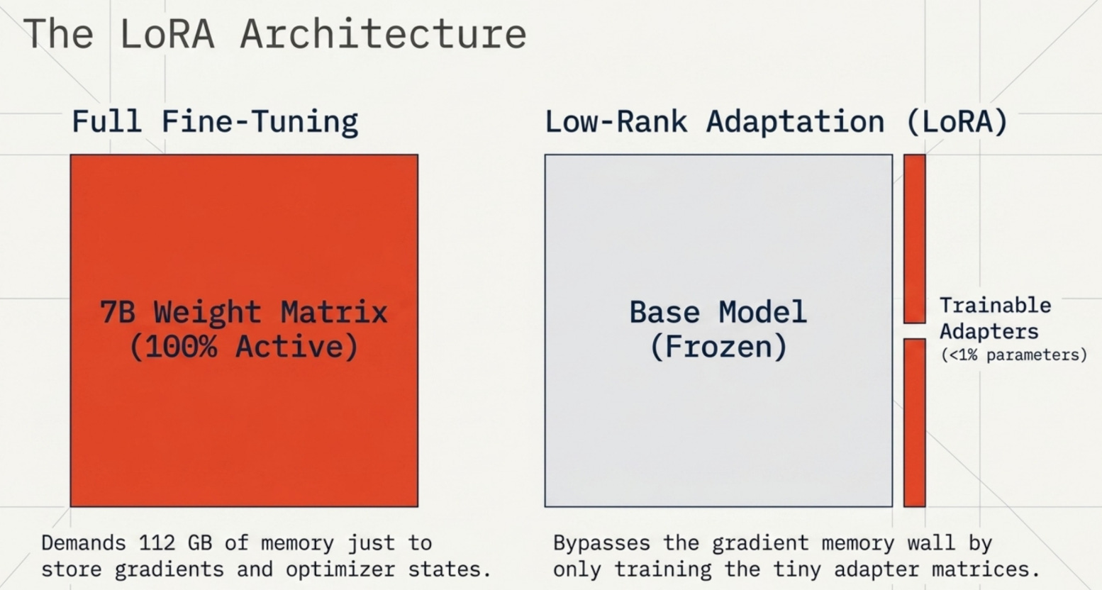
Full fine-tuning means updating every single weight in a model during training. For a 7B model, that’s 7 billion gradients computed and stored per step, plus the Adam optimizer’s momentum and variance terms. The total memory for full FP32 fine-tuning is approximately 112 GB for a 7B model, which requires at minimum two A100 80GB GPUs.
LoRA takes a completely different approach, motivated by a hypothesis that the weight updates needed for task-specific fine-tuning have low intrinsic rank. Instead of updating the full weight matrix W directly, LoRA freezes W and trains two small matrices A and B whose product approximates the update.
# Regular weight matrix W: shape [d_out, d_in]
# LoRA modification: W_effective = W + B @ A
# where A: [r, d_in] and B: [d_out, r], r << min(d_in, d_out)

# For a typical transformer layer: d_in = d_out = 4096
# Full matrix: 4096 * 4096 = 16.8M parameters
# LoRA rank 8: A (8 * 4096 = 32K) + B (4096 * 8 = 32K) = 64K parameters
# That's 0.38% of the original parameter count
In practice, LoRA reduces trainable parameters to about 0.1% to 1% of the full model, which dramatically shrinks gradient and optimizer memory. The frozen base model doesn’t need gradients at all. Only the tiny LoRA adapters do.
The natural next step is to combine this with quantization: freeze the base model in INT4 or INT8, and train only the BF16 LoRA adapters. This is exactly what QLoRA does.
QLoRA: Putting It All Together
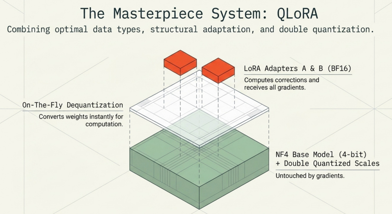
QLoRA (Quantized Low-Rank Adaptation) combines three techniques: NF4 quantization for the frozen base model, LoRA adapters in BF16 for training, and double quantization to reduce the scale factor overhead. Together, they make fine-tuning 70B models feasible on consumer hardware.
The memory breakdown for a 7B model trained with QLoRA versus alternatives:
Model           Full FP32    Full BF16    LoRA BF16    QLoRA NF4
-------------------------------------------------------------------
7B model         112.0 GB      84.0 GB      14.1 GB       3.6 GB
13B model        208.0 GB     156.0 GB      26.1 GB       6.6 GB
70B model       1120.0 GB     840.0 GB     140.7 GB      35.7 GB
A 70B model that required 1120 GB for full FP32 training fits into 35.7 GB with QLoRA. That fits on a single A100 80GB GPU with headroom to spare.
The workflow during QLoRA training:
Load the base model in NF4. Weights are stored as 4-bit integers with per-block scale factors. The base model uses roughly 0.5 bytes per parameter.
Add LoRA adapters in BF16. For each target layer (usually query, key, value, and output projection matrices in attention), initialize A and B matrices with small random values. These are tiny (< 1% of total params) but stored in full BF16 precision.
Forward pass. When computing through a quantized layer, dequantize the NF4 weights on the fly to BF16 for the matrix multiplication. Compute the LoRA correction (B @ A) and add it to the output. The dequantization is fast and happens in-place, without storing a separate FP32 copy.
Backward pass. Only the LoRA adapters have requires_grad=True. Gradients flow through the LoRA path and back through the dequantized matrix operations. The base NF4 weights are never updated.
Save adapters only. At the end of training, you save just the LoRA adapter weights (a few hundred MB), not the full base model. These adapters can be merged back at inference time or loaded separately.
Training vs Inference Tradeoffs
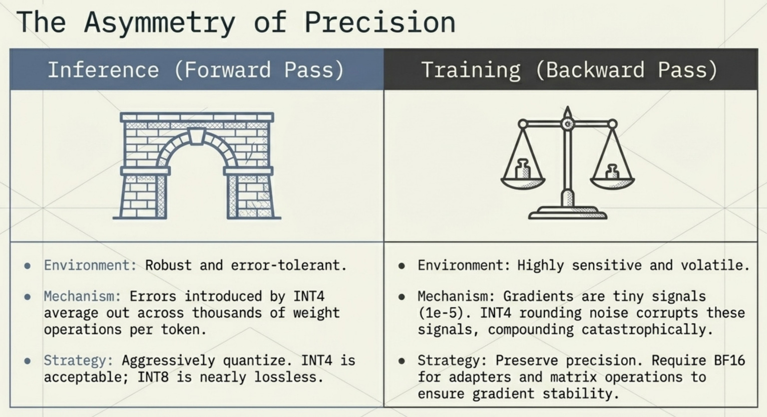
One of the most important things to understand about quantization is that its effects are not symmetric between training and inference. What works beautifully for one can be disastrous for the other.
Inference is much more tolerant of quantization. You’re running a single forward pass, computing outputs from inputs. The errors introduced by INT8 or INT4 quantization average out across the thousands of weight operations that contribute to each output token. Empirically, INT8 inference on 7B+ models produces outputs that are nearly indistinguishable from FP16 inference on most benchmarks. INT4 inference shows measurable but acceptable perplexity increases on language modeling tasks.
Training is entirely different. The backward pass computes gradients by propagating small error signals backward through the entire network. These signals are often tiny (on the order of 1e-5 or smaller for deep layers) and need to be accumulated precisely across thousands of optimization steps. Quantization noise that’s inconsequential for a single prediction becomes catastrophic when it corrupts gradient signals that determine the direction of weight updates.
This is why QLoRA specifically uses:
NF4 for the frozen base model weights (inference-only, high compression is fine)
BF16 for the trainable LoRA adapters (training mode, needs precision for gradient accumulation)
BF16 for computation (matrix multiplications dequantize to BF16 on the fly, giving precise forward and backward passes)
The practical implication: always quantize for inference, be very selective about what you quantize for training. The 35.7 GB QLoRA number for a 70B model is an inference-focused estimate. The actual training memory will be slightly higher due to activation checkpointing and intermediate BF16 buffers, but it stays within the realm of single-GPU feasibility.
Limitations of Quantization
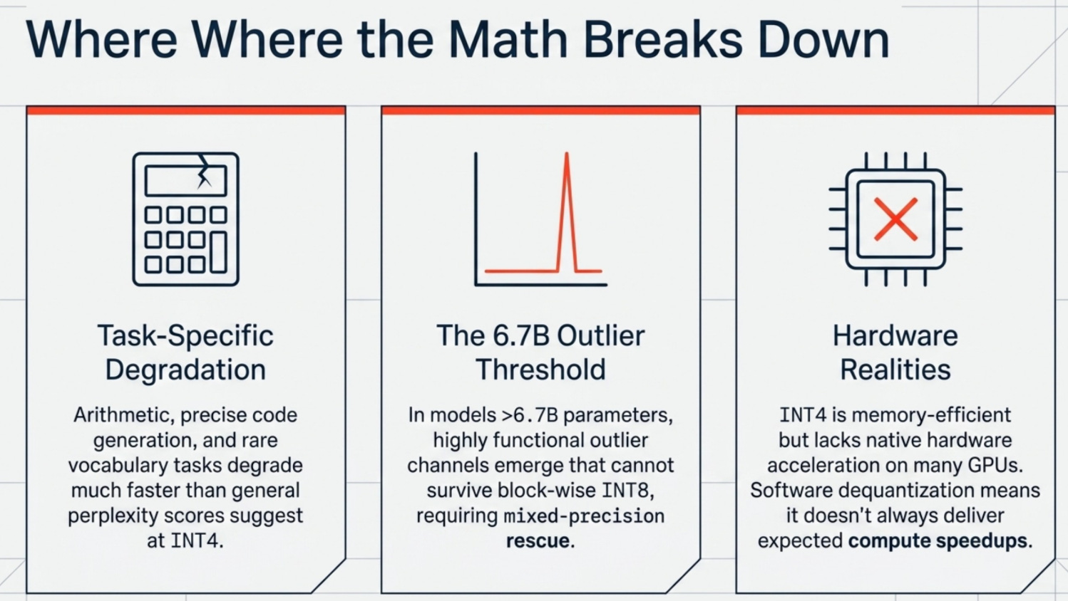
Quantization is a powerful tool, but it isn’t magic. Understanding where it breaks down is as important as knowing how to apply it.
Accuracy degradation on specific tasks. While average perplexity losses from INT4 quantization are modest (typically 1-3% on general benchmarks), certain tasks are disproportionately affected. Reasoning chains that require arithmetic, code generation with precise syntax, and tasks involving rare vocabulary can degrade significantly more than benchmark averages suggest. This is because those tasks depend on specific weight patterns that might be compressed out by aggressive quantization.
Outlier sensitivity. Even with block-wise quantization, certain layers in large models have activation outliers so extreme that they corrupt entire blocks. Research on LLM.int8() found that these outlier features emerge at scales above 6.7B parameters and require mixed-precision handling: keeping the most critical weight channels in FP16 while quantizing the rest to INT8.
Hardware compatibility. Not all quantization formats are hardware-accelerated. INT8 matrix operations are native on NVIDIA A100s and newer hardware, but INT4 and NF4 typically require software dequantization to FP16 before the actual matrix multiply. This means INT4 is memory-efficient but doesn’t always deliver the compute speedup you’d expect from having half the bits to process.
Quantization-aware fine-tuning complexity. Deploying a quantized model that was quantized post-training is straightforward. But if you want maximum accuracy at a given bit width, you need quantization-aware training (QAT), which adds significant complexity to the training pipeline and requires careful calibration of quantization parameters.
Latest Innovations
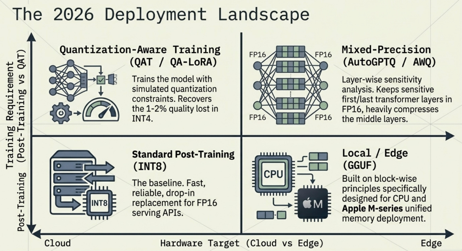
The quantization research landscape in 2025 and 2026 has moved beyond the foundational techniques and into increasingly sophisticated territory.
Quantization-Aware Training (QAT) trains the model with simulated quantization applied during the forward pass. The model learns to work within the constraints of reduced precision, which typically recovers 1-2% quality compared to post-training quantization. Models trained with QAT can often be deployed at INT4 with near-FP16 quality.
QA-LoRA extends QLoRA by making the LoRA adapters quantization-aware. Instead of training BF16 adapters alongside a frozen NF4 model, QA-LoRA trains adapters whose outputs are designed to compensate for the quantization error in the frozen weights. This produces adapters that perform better when the final merged model is deployed in INT4.
Mixed-precision pipelines move away from applying the same quantization uniformly across all layers. Research has shown that the first and last layers of a transformer are disproportionately sensitive to quantization and should be kept at higher precision (FP16 or BF16), while the middle layers can tolerate INT4. Tools like AutoGPTQ and llama.cpp implement layer-wise sensitivity analysis to automatically determine the optimal precision per layer.
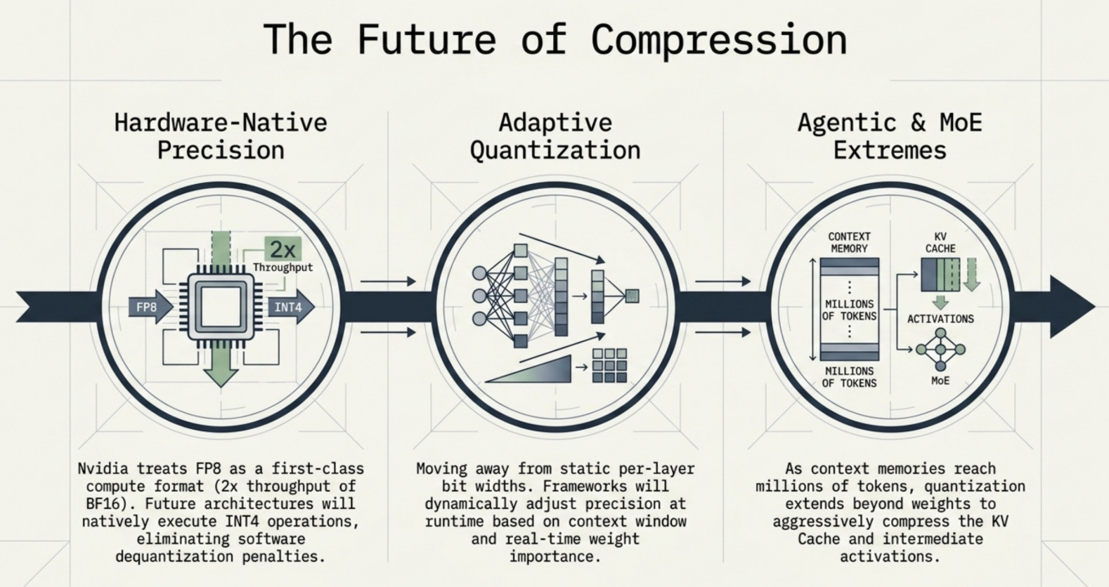
Hardware-aware quantization designs quantization strategies around the specific arithmetic units of the target hardware. NVIDIA’s FP8 format (introduced in the H100) has 8-bit floating-point with configurable exponent/mantissa splits, allowing different FP8 variants for weights versus activations. The H100’s native FP8 tensor cores achieve 2x the throughput of BF16 with minimal accuracy loss, effectively giving you INT8-like memory efficiency with floating-point numerical properties.
Activation quantization extends compression beyond just weights to the intermediate activations computed during inference. Since activations are the bottleneck for KV cache memory in long-context inference, quantizing them to INT8 or FP8 can dramatically reduce the memory cost of serving long-context requests.
Real-World Use Cases
The techniques discussed here are not academic exercises. They’re actively deployed in production systems that handle millions of requests per day.
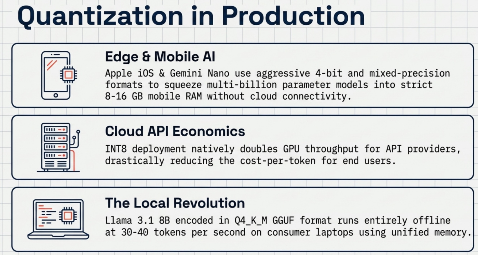
Edge and mobile AI. Quantization is what makes it possible to run capable language models on phones and tablets. Apple’s on-device AI models in iOS 18 use aggressive 4-bit quantization to fit multi-billion parameter models within the 8-16 GB memory constraints of mobile devices. Google’s Gemini Nano uses mixed-precision quantization to run on Android phones without cloud connectivity.
Cost-efficient cloud APIs. API providers serving inference at scale quantize their models by default. INT8 inference roughly doubles the throughput per GPU compared to BF16, directly translating to lower cost per token for users. INT4 inference doubles it again, though with more quality scrutiny required.
Local deployment on consumer hardware. Tools like llama.cpp, Ollama, and LM Studio use GGUF quantization (a format built on top of block-wise quantization principles) to run 7B and 13B models on MacBook M-series chips and consumer GPUs with 8-16 GB VRAM. The Llama 3.1 8B model in Q4_K_M GGUF format runs at around 30-40 tokens per second on an M2 MacBook Pro, entirely locally, entirely offline.
Domain-specific fine-tuning on a budget. QLoRA has democratized fine-tuning by making it accessible on single GPUs. Research labs, startups, and individual developers routinely fine-tune 7B and 13B models on domain-specific datasets using single A100 or 3090 GPUs that cost a few hundred dollars per month to rent. The fine-tuned models perform comparably to much larger general-purpose models on their specific task.
Future of Quantization
The trajectory of quantization research points toward three converging directions.
Adaptive quantization will become the standard. Instead of choosing a single bit width for an entire model, future systems will dynamically adjust precision based on the importance of each weight, the uncertainty in the model’s outputs, and the computational budget available at runtime. Early work on importance-weighted quantization and dynamic precision has shown significant quality improvements over static per-layer approaches.
Hardware-native low precision will blur the line between quantization as a compression technique and quantization as a native arithmetic format. NVIDIA’s H100 and H200 already treat FP8 as a first-class compute format. Future accelerators are likely to include native support for INT4 tensor operations, eliminating the dequantization overhead that currently makes INT4 slower than its memory savings would suggest.
Integration with mixture-of-experts and agentic systems will introduce new quantization challenges. MoE models activate only a subset of experts for each token, which means the optimal quantization strategy may differ between active and inactive experts. Agentic LLMs that need to cache long context histories will push activation quantization to new extremes as context windows extend to millions of tokens.
The direction is clear: quantization is moving from a post-hoc compression trick to a foundational design principle that shapes how models are trained, stored, and served from the ground up.
Conclusion
Quantization is what turns powerful models into usable systems. It’s the difference between a research artifact that requires a data center and a production tool that runs on a laptop. The mathematics are elegant: by understanding the structure of LLM weight distributions and choosing precision formats that match that structure, you can compress models by 4x to 8x with surprisingly little quality loss.
The key ideas to carry forward:
INT8 quantization reduces memory by 4x from FP32 with negligible quality loss. It’s the baseline for production inference.
Block-wise quantization solves the outlier problem that makes naive INT8 fail on large models, delivering 4x lower reconstruction error.
NF4 data type places quantization levels at normal distribution quantiles, optimizing 4-bit precision for the actual shape of transformer weight distributions.
Double quantization compresses the scale factors themselves, eliminating most of the overhead introduced by block-wise approaches.
QLoRA combines all three to make fine-tuning a 70B model feasible on a single GPU, reducing training memory from 1120 GB to under 36 GB.
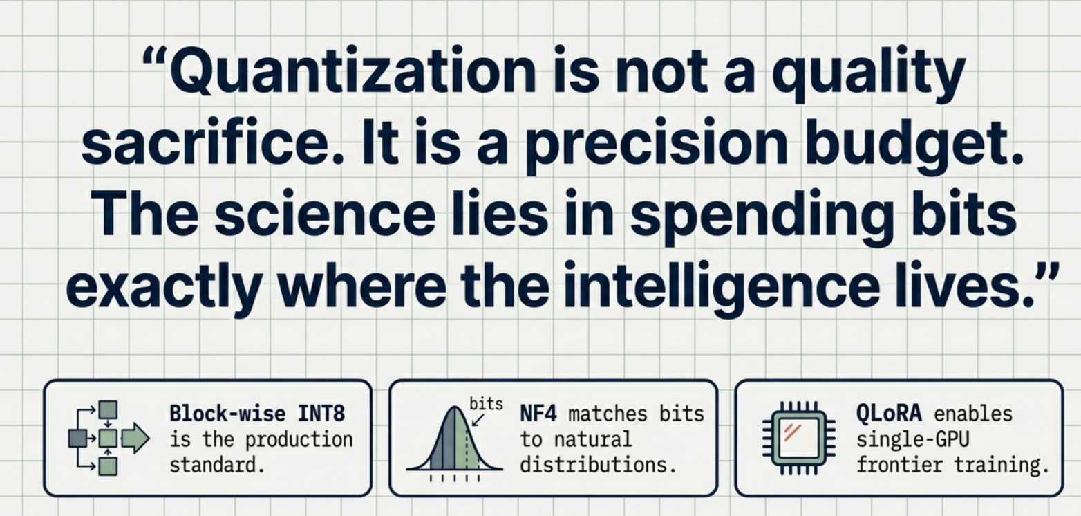
The right way to think about quantization is not as a quality sacrifice but as a precision budget. You have a fixed number of bits available, and quantization is the science of spending that budget wisely across the weight distribution that carries your model’s intelligence.
Frequently Asked Questions
Does INT4 quantization hurt model quality significantly?
At INT4, you see a mean absolute reconstruction error roughly 15x higher than INT8 (0.109 vs 0.006 in our benchmarks). For general language tasks, this translates to a 1-3% perplexity increase, which is noticeable but acceptable for most applications. Tasks requiring precise arithmetic or rare vocabulary suffer more. INT8 is the safer default; INT4 is for memory-constrained scenarios.
Can I quantize any model, or only specific architectures?
Post-training quantization works on any transformer-based model. Block-wise and NF4 quantization are architecture-agnostic and depend only on the weight distribution properties, which are consistent across GPT, Llama, Mistral, and similar architectures. Models with unusual weight distributions (after heavy fine-tuning or with non-standard initialization) may require per-layer calibration.
What is the difference between quantization and pruning?
Quantization reduces the precision used to represent each weight. Pruning removes weights entirely by setting them to zero. They’re complementary techniques: pruning reduces the number of operations, while quantization reduces the memory and compute cost of each operation. Many production pipelines combine both, though quantization alone typically delivers better quality-to-compression ratios for LLMs.
How much GPU memory do I actually need for QLoRA fine-tuning?
Our estimates: a 7B model needs ~3.6 GB for the quantized weights plus ~0.5 GB for LoRA adapters and optimizer states, putting you comfortably on a 16 GB consumer GPU like the RTX 4080. A 13B model needs ~6.6 GB total, still fitting on 16 GB. A 70B model needs ~35.7 GB, requiring an A100 40 GB or H100 80 GB.
Is quantization the same as model distillation?
No. Quantization compresses an existing model by reducing weight precision while keeping the same architecture. Distillation trains a smaller model to mimic the outputs of a larger model, resulting in a genuinely smaller neural network. Quantization is faster and requires no training data. Distillation requires training and a teacher model but can achieve better quality at very small model sizes.
Image credits: Google NotebookLM and Nano Banana